Gromacs Quick Start
GROMACS Quick Start
Official Documentation:
Gromacs Server and Environment:
source /usr/local/gromacs/bin/GMXRCwget https://repo.anaconda.com/miniconda/Miniconda3-latest-Linux-x86_64.shchmod +x Miniconda3-latest-Linux-x86_64.sh./Miniconda3-latest-Linux-x86_64.sh (answer yes to initialize Minicoda3)conda install numpy scipy matplotlib pandasconda deactivateconda activateGromacs Command
gmkExamples:
gmx -h (print help)gmk -v (show version)gmx help [module] (documentation of a module)Example 1: Lysozyme
Prepare structure and topology files
mkdir lysozymecd lysozymegetpdb 1akiconda deactivatepymol 1aki.pdbconda activategrep -v HOH 1aki.pdb > 1aki_clean.pdbgmx pdb2gmx -f 1aki_clean.pdb -o 1AKI_processed.gro -water spcegmx help pdb2gmx- topol.top Topology file defines atom and bond parameters.
- posre.itp Position restraint file
Define the simulation box and solvent
Step 1: Define the box dimensions using the editconf module
gmx editconf -f 1AKI_processed.gro -o 1AKI_newbox.gro -c -d 1.0 -bt cubic
This command use module editconf to center and define a box.
- -f 1AKI_processed.gro: Input file
- -o 1AKI_newbox.gro: Output file, the box is 0,0,0 and the coordinates at the bottom line
- -c: center the box
- -d 1.0: Leave at least 1 nm at the edge
- -bt cubic: Use cubic box. There are other choices such as rhombic dodecahedron.
Step 2: Fill the box with water using the solvate module
gmx solvate -cp 1AKI_newbox.gro -cs spc216.gro -o 1AKI_solv.gro -p topol.top- -cp 1AKI_newbox.pro: Configuration of the protein from the named file
- -cs spc216.gro: Configuration of the solvent. Spc216.gro is a generic equilibrated 3-point solvent model good for SPC, SPC/E, or TIP3P water.
- -o 1AKI_solv.gro: Output file name
- -p topol.top: Topology file name. Solvate module will update this file to include both protein molecule and solvate (SOL) line
Add ions
In topology file [ atom ] section, the protein total charge is calculated. The charge at the end of this section is the net charge.
1960 opls_272 129 LEU O2 682 -0.8 15.9994 ; qtot 8In this example, the net charge is 8.
In MD simulation, we need to balance the charge with ions so that we have a neutral system. This is a two step procedure.
Step 1: Prepare a run input file (extension .tpr) for genion module
MD parameter file ions.mdp contains instructions for Gromacs Preprocessor module grompp to assemble coordinates and topology into an atomic-level input .tpr file.
Sample ions.mdp file
; ions.mdp - used as input into grompp to generate ions.tpr
; Parameters describing what to do, when to stop and what to save
integrator  = steep         ; Algorithm (steep = steepest descent minimization)
emtol       = 1000.0        ; Stop minimization when the maximum force < 1000.0 kJ/mol/nm
emstep      = 0.01          ; Minimization step size
nsteps      = 50000         ; Maximum number of (minimization) steps to perform

; Parameters describing how to find the neighbors of each atom and how to calculate the interactions
nstlist         = 1         ; Frequency to update the neighbor list and long range forces
cutoff-scheme	= Verlet    ; Buffered neighbor searching
ns_type         = grid      ; Method to determine neighbor list (simple, grid)
coulombtype     = cutoff    ; Treatment of long range electrostatic interactions
rcoulomb        = 1.0       ; Short-range electrostatic cut-off
rvdw            = 1.0       ; Short-range Van der Waals cut-off
pbc             = xyz       ; Periodic Boundary Conditions in all 3 dimensions
This mdp file tells Gromacs to run an energy minimization.
gmx grompp -f ions.mdp -c 1AKI_solv.gro -p topol.top -o ions.tpr
- Module grompp is a gromacs preprocessor. Its job is to make a .tpr file.
- -f ions.mdp: Read instruction from ions.mdp file.
- -c 1AKI_solv.gro: Coordinates file
- -p topol.top: Topology file
- -o ions.tpr: Output file. This is an atomic level input file with coordinates and topology all assembled. It's going to be the input of MD simulation. In this case, it will be the input of ion adding module's input file.
Step 2: Use module genion to replace some water molecules with ions
gmx genion -s ions.tpr -o 1AKI_solv_ions.gro -p topol.top -pname NA -nname CL -neutral
- -s ions.tpr: Specify structure file ions.tpr.
- -o 1AKI_solv_ions.gro: Write to this output file.
- -p topol.top: Update topology file to reflect the removal of water and addition of ions.
- -pname NA: Use NA for position ion.
- -nname CL: Use CL for negative ion.
- -neutral: Neutralize the system. In this case, it will replace 8 waters by CL- to offset the 8 positive net charge.
When prompted, choose option 13 SOL so module genion will replace solvent molecules.
After this step, the topol.top file will include CL in its [ molecules ] section:
[ molecules ]
; Compound #mols
Protein_chain_A 1
SOL 10636
CL 8
Energy minimization:
We have a solvated and charge neutral system by now in coordinates file 1AKI_solv_ions.gro with the molecule toplogy in file topol.top. Before we run production MD, we have a few more prepartion steps:
- Energy minimization: Remove structure clashes.
- Equilibration: Move the structure from high energy state to equilibrated state.
Similar to add ions step, we need to make a MD include-all atomic level .tpr file, with 3 pieces of information:
- .mdp file: MD parameter file that serves as instruction script
- .gro file: Gromacs coordinate file
- .top file: Topology file
Sample minim.mdp file:
; minim.mdp - used as input into grompp to generate em.tpr
; Parameters describing what to do, when to stop and what to save
integrator  = steep         ; Algorithm (steep = steepest descent minimization)
emtol       = 1000.0        ; Stop minimization when the maximum force < 1000.0 kJ/mol/nm
emstep      = 0.01          ; Minimization step size
nsteps      = 50000         ; Maximum number of (minimization) steps to perform

; Parameters describing how to find the neighbors of each atom and how to calculate the interactions
nstlist         = 1         ; Frequency to update the neighbor list and long range forces
cutoff-scheme   = Verlet    ; Buffered neighbor searching
ns_type         = grid      ; Method to determine neighbor list (simple, grid)
coulombtype     = PME       ; Treatment of long range electrostatic interactions
rcoulomb        = 1.0       ; Short-range electrostatic cut-off
rvdw            = 1.0       ; Short-range Van der Waals cut-off
pbc             = xyz       ; Periodic Boundary Conditions in all 3 dimensions
This .mdp file is the same as ions.mdp except the coulombtype. PME is Fast smooth Particle-Mesh Ewald (SPME) electrostatics, more accurate than cutoff in ions.mdp.
gmx grompp -f minim.mdp -c 1AKI_solv_ions.gro -p topol.top -o em.tpr
- grompp: Gromacs preprocessor to assemble .gro and .top files.
- -f minim.mdp: MD parameter file
- -c 1AKI_solv_ions.gro: Coordinate file
- -p topol.top: Toplogy file
- -o em.tpr: Output file
Once the em.tpr is ready, we can pass it to mdrun module to run an energy minimization.
gmx mdrun -v -deffnm em
- mdrun: MD simulation module
- -v: Verbose mode
- -deffnm: Define file names of the input and output. If you did not name your grompp output "em.tpr," you will have to explicitly specify its name with the mdrun -s flag.
Since we passed the model em in, mdrun takes em.tpr as input and writes out 4 files that start with em. Gromacs will detect CPU and uses OpenMP to run on maximum available threads. If you would like control the number of threads manually, use option
-ntomp
For example
gmx mdrun -v -ntomp 8 -deffnm em
Will uses 8 threads.
This step produces output files as following:
(base) jmao@gromacs:~/demo/lysozyme$ ls -lt
total 9044
-rw-rw-r-- 1 jmao jmao 305030 Oct 18 13:32 em.log
-rw-rw-r-- 1 jmao jmao 1524475 Oct 18 13:32 em.gro
-rw-rw-r-- 1 jmao jmao 406632 Oct 18 13:32 em.trr
-rw-rw-r-- 1 jmao jmao 129712 Oct 18 13:32 em.edr
-rw-rw-r-- 1 jmao jmao 848248 Oct 18 13:27 em.tpr
These files are:
- em.log: ASCII-text log file of the EM process
- em.edr: Binary energy file
- em.trr: Binary full-precision trajectory
- em.gro: Energy-minimized structure
The energy file is a binary file and not directly viewable. To see the minimization process and evaluate the convergence quality, we can convert this energy file to a plot.
gmx energy -f em.edr -o potential.xvg
- energy: Energy module extracts energy components from an energy file.
- -f em.edr: The energy file as input
- -o potential.xvg: Write out the energy trace plot to this file.
When prompted, enter "10 0". "10" is to select potential and "0" is to end the input.
To view the plot, run
xmgrace potential.xvg
You need to enable X11 forwarding when you ssh to the server. That is to use "-X option in ssh command such as "ssh -X username@serverIP"
Energy equilibration:
While energy minimization brings the structure to a low energy state quickly, we are not at the equilibrated state at a desired temperature, and the equilibrated state including the solvent and solvate.
The eqilibration is often conducted in two phases.
The first phase is conducted under an NVT ensemble (constant Number of particles, Volume, and Temperature). In NVT, the temperature of the system should reach a plateau at the desired value. Typically, 50-100 ps should suffice.
The second phase is conducted under an NPT ensemble (constant Number of particles, Pressure, and Temperature). After NPT euilibration, the presure and density might fluctuate, but the running average should be stable. This phase generally requires longer to reach equilibration than NVT.
Phase 1: NVT equilibration
Again we need 3 input files to assemble the atomic-level md .tpr file
- .mdp file: MD parameter file that serves as instruction script
- .gro file: Gromacs coordinate file. Use em.gro from energy minimization
- .top file: Topology file. This file keeps the same name topol.top.
nvt.mdp
title                   = OPLS Lysozyme NVT equilibration
define                  = -DPOSRES  ; position restrain the protein
; Run parameters
integrator              = md        ; leap-frog integrator
nsteps                  = 50000     ; 2 * 50000 = 100 ps
dt                      = 0.002     ; 2 fs
; Output control
nstxout                 = 500       ; save coordinates every 1.0 ps
nstvout                 = 500       ; save velocities every 1.0 ps
nstenergy               = 500       ; save energies every 1.0 ps
nstlog                  = 500       ; update log file every 1.0 ps
; Bond parameters
continuation            = no        ; first dynamics run
constraint_algorithm    = lincs     ; holonomic constraints
constraints             = h-bonds   ; bonds involving H are constrained
lincs_iter              = 1         ; accuracy of LINCS
lincs_order             = 4         ; also related to accuracy
; Nonbonded settings
cutoff-scheme           = Verlet    ; Buffered neighbor searching
ns_type                 = grid      ; search neighboring grid cells
nstlist                 = 10        ; 20 fs, largely irrelevant with Verlet
rcoulomb                = 1.0       ; short-range electrostatic cutoff (in nm)
rvdw                    = 1.0       ; short-range van der Waals cutoff (in nm)
DispCorr                = EnerPres  ; account for cut-off vdW scheme
; Electrostatics
coulombtype             = PME       ; Particle Mesh Ewald for long-range electrostatics
pme_order               = 4         ; cubic interpolation
fourierspacing          = 0.16      ; grid spacing for FFT
; Temperature coupling is on
tcoupl                  = V-rescale             ; modified Berendsen thermostat
tc-grps                 = Protein Non-Protein   ; two coupling groups - more accurate
tau_t                   = 0.1     0.1           ; time constant, in ps
ref_t                   = 300     300           ; reference temperature, one for each group, in K
; Pressure coupling is off
pcoupl                  = no        ; no pressure coupling in NVT
; Periodic boundary conditions
pbc                     = xyz       ; 3-D PBC
; Velocity generation
gen_vel                 = yes       ; assign velocities from Maxwell distribution
gen_temp                = 300       ; temperature for Maxwell distribution
gen_seed                = -1        ; generate a random seed
Assemble the tpr file:
gmx grompp -f nvt.mdp -c em.gro -r em.gro -p topol.top -o nvt.tpr
This command is similar to commands used in adding ions and energy minimization. The instruction parameter file mdp is different. Some parameters worth attention are:
- nsteps=5000 and dt=0.2: They combined to define the run time 100 ps
- pcoupl= no: No pressure coupling for NVT equilibration
- ref_t=300: Temperature at 300K
This will generate file nvt.tpr as input for mdrun:
gmx mdrun -deffnm nvt
The output files have names as nvt.*
To check the temperature convergence, use the energy module choice 16.
gmx energy -f nvt.edr -o temperature.xvg
Type "16 0" at the prompt to select Temperature. Use xmgrace temperature.xvg to view the system temperature.
Phase 2: NPT equilibration
We need 3 input files to assemble the atomic-level md .tpr file
- .mdp file: MD parameter file that serves as instruction script
- .gro file: Gromacs coordinate file. Use nvt.gro from NVT equilibration
- .top file: Topology file. This file keeps the same name topol.top.
In ntp.mdp file:
title                   = OPLS Lysozyme NPT equilibration
define                  = -DPOSRES  ; position restrain the protein
; Run parameters
integrator              = md        ; leap-frog integrator
nsteps                  = 50000     ; 2 * 50000 = 100 ps
dt                      = 0.002     ; 2 fs
; Output control
nstxout                 = 500       ; save coordinates every 1.0 ps
nstvout                 = 500       ; save velocities every 1.0 ps
nstenergy               = 500       ; save energies every 1.0 ps
nstlog                  = 500       ; update log file every 1.0 ps
; Bond parameters
continuation            = yes       ; Restarting after NVT
constraint_algorithm    = lincs     ; holonomic constraints
constraints             = h-bonds   ; bonds involving H are constrained
lincs_iter              = 1         ; accuracy of LINCS
lincs_order             = 4         ; also related to accuracy
; Nonbonded settings
cutoff-scheme           = Verlet    ; Buffered neighbor searching
ns_type                 = grid      ; search neighboring grid cells
nstlist                 = 10        ; 20 fs, largely irrelevant with Verlet scheme
rcoulomb                = 1.0       ; short-range electrostatic cutoff (in nm)
rvdw                    = 1.0       ; short-range van der Waals cutoff (in nm)
DispCorr                = EnerPres  ; account for cut-off vdW scheme
; Electrostatics
coulombtype             = PME       ; Particle Mesh Ewald for long-range electrostatics
pme_order               = 4         ; cubic interpolation
fourierspacing          = 0.16      ; grid spacing for FFT
; Temperature coupling is on
tcoupl                  = V-rescale             ; modified Berendsen thermostat
tc-grps                 = Protein Non-Protein   ; two coupling groups - more accurate
tau_t                   = 0.1     0.1           ; time constant, in ps
ref_t                   = 300     300           ; reference temperature, one for each group, in K
; Pressure coupling is on
pcoupl                  = Parrinello-Rahman     ; Pressure coupling on in NPT
pcoupltype              = isotropic             ; uniform scaling of box vectors
tau_p                   = 2.0                   ; time constant, in ps
ref_p                   = 1.0                   ; reference pressure, in bar
compressibility         = 4.5e-5                ; isothermal compressibility of water, bar^-1
refcoord_scaling        = com
; Periodic boundary conditions
pbc                     = xyz       ; 3-D PBC
; Velocity generation
gen_vel                 = no        ; Velocity generation is off
Some differences over nvt.mdp are:
- continuation = yes: This says we will use the coordinates from
- pcoupl=Parrinello-Rahman: Presure coupling for NPT
gmx grompp -f npt.mdp -c nvt.gro -r nvt.gro -t nvt.cpt -p topol.top -o npt.tpr
In this command, an extra option -t nvt.cpt is added because we specified continuation=yes. We use the checkpoint file from NVT phase.
After we have npt.tpr, we run the NPT phase of equilibration:
gmx mdrun -deffnm npt
The output files have names npt.*
Now check the presure:
gmx energy -f npt.edr -o pressure.xvg
Chose option "18 0" to select Pressure.
View the plot:
xmgrace pressure.xvg
Unlike the temperature, presure varies widely. This is normal behavior for MD simulation though, as long as the running average of presure is steady.
To generate running average in xmgrace, Go to Data -> Transformation -> Running average, select a set (Set 0 in our case) and specify length of average (10 ps in our case)
Production MD
The system is ready to run production MD after the equilibration to the desired tenperature. We will run MD for longer time, usually in nano seconds to collect statistically meaningful results.
md.mdp
title                   = OPLS Lysozyme NPT equilibration
; Run parameters
integrator              = md        ; leap-frog integrator
nsteps                  = 500000    ; 2 * 500000 = 1000 ps (1 ns)
dt                      = 0.002     ; 2 fs
; Output control
nstxout                 = 0         ; suppress bulky .trr file by specifying
nstvout                 = 0         ; 0 for output frequency of nstxout,
nstfout                 = 0         ; nstvout, and nstfout
nstenergy               = 5000      ; save energies every 10.0 ps
nstlog                  = 5000      ; update log file every 10.0 ps
nstxout-compressed      = 5000      ; save compressed coordinates every 10.0 ps
compressed-x-grps       = System    ; save the whole system
; Bond parameters
continuation            = yes       ; Restarting after NPT
constraint_algorithm    = lincs     ; holonomic constraints
constraints             = h-bonds   ; bonds involving H are constrained
lincs_iter              = 1         ; accuracy of LINCS
lincs_order             = 4         ; also related to accuracy
; Neighborsearching
cutoff-scheme           = Verlet    ; Buffered neighbor searching
ns_type                 = grid      ; search neighboring grid cells
nstlist                 = 10        ; 20 fs, largely irrelevant with Verlet scheme
rcoulomb                = 1.0       ; short-range electrostatic cutoff (in nm)
rvdw                    = 1.0       ; short-range van der Waals cutoff (in nm)
; Electrostatics
coulombtype             = PME       ; Particle Mesh Ewald for long-range electrostatics
pme_order               = 4         ; cubic interpolation
fourierspacing          = 0.16      ; grid spacing for FFT
; Temperature coupling is on
tcoupl                  = V-rescale             ; modified Berendsen thermostat
tc-grps                 = Protein Non-Protein   ; two coupling groups - more accurate
tau_t                   = 0.1     0.1           ; time constant, in ps
ref_t                   = 300     300           ; reference temperature, one for each group, in K
; Pressure coupling is on
pcoupl                  = Parrinello-Rahman     ; Pressure coupling on in NPT
pcoupltype              = isotropic             ; uniform scaling of box vectors
tau_p                   = 2.0                   ; time constant, in ps
ref_p                   = 1.0                   ; reference pressure, in bar
compressibility         = 4.5e-5                ; isothermal compressibility of water, bar^-1
; Periodic boundary conditions
pbc                     = xyz       ; 3-D PBC
; Dispersion correction
DispCorr                = EnerPres  ; account for cut-off vdW scheme
; Velocity generation
gen_vel                 = no        ; Velocity generation is off
This file is largely the same as NPT equilibration, but runs longer and saves more frequently.
gmx grompp -f md.mdp -c npt.gro -t npt.cpt -p topol.top -o md_0_1.tpr
gmx mdrun -deffnm md_0_1
This run takes long time.
Analysis
Trajectory conversion:
As molecules will shift out of the box during long simulation, this is a psot-processing step to strip out coordinates, correct for periodicity, or manually alter the trajectory (time units, frame frequency, etc).
gmx trjconv -s md_0_1.tpr -f md_0_1.xtc -o md_0_1_noPBC.xtc -pbc mol -center
Select "1 Protein" to be centered and "0 System" to be written out.
- trjconv: Gromacs trajectory convert module.
- -s md_0_1.tpr: all-atom run input file
- -f md_0_1.xtc: trajectory file as input
- -o md_0_1_noPBC.xtc: converted trajectory file as output
- -pbc mol: Periodical Boundary Correction (PBC) treatment method to use molecule
- -center: center atoms in box
All analysis will be conducted on the converted trajectory md_0_1_noPBC.xtc.
RMSD - Structure stablity
RMSD module can calculate the RMSD between a trajectory and a reference structure.
gmx rms -s md_0_1.tpr -f md_0_1_noPBC.xtc -o rmsd.xvg -tu ns
Select "4 Backbone" for fitting and "4 Backbone" for RMSD calculation.
- -s md_0_1.tpr: all-atom run input file
- -f md_0_1_noPBC.xtrc: trajectory file
- -o rmsd.xvg: write rmsd plot
- -tu ns: specify ns as time unit
Write out snapshots in odb format for viewing
Write out the whole structure at 100 ps
gmx trjconv -s md_0_1.tpr -f md_0_1.xtc -dump 100 -o snapshot100.pdb
Choose "0 System" for the whole system.
Write out the protein structure at every 2 ps
gmx trjconv -s md_0_1.tpr -f md_0_1.xtc -dt 2 -o snapshot.pdb
Choose "1 Protein" for the protein only.
Multiple frames are marked as models in the output pdb file. When viewing the structure with Pymol, the "play" button will show the frames as a movie sequence.
Example 2: Building Biphasic Systems
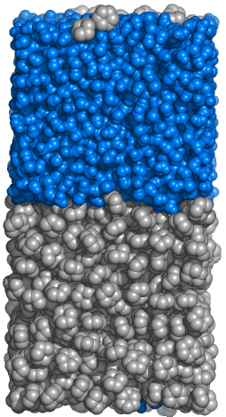
Make a heterogeneous biphasic system composed of hydrophobic (cyclohexane) and hydrophilic (water) layers.
This example illustrates the procedure of making a new molecule that the Gromacs doesn't know.