How does changing MCCE's parameters change accuracy? (under construction)

MCCE offers a wide range of customizable parameter that influence the accuracy of its pKa predictions. Some major options include varying the internal dielectric constants, numerical Poisson-Boltzmann solvers, Van der Waal functions, conformer sampling level, and explicit crystal water inclusion/removal (implicit/explicit). Each of these options or combinatoric assortments of these options can significantly impact MCCE's free energy model, and in turn, affects its pKa predictions. In this study, we systematically evaluate how these parameter choices affect MCCE's calculated pKa values against experimental benchmark values. 

Here, we use a set of 36 PDB files sourced from RCSB.org, see PDB Benchmark Files.txt. These PDB files were chosen for their varying sizes, as well as the amount of experimental data available for their residue pKa values. You can find the sources for the experimental pKas in this file: pkdbv1_WT_pkas.csv (change this later to be a citation probably)

Note that the starting and ending residues of protein chains are re-named to NTR and CTR, respectively. At time of writing, MCCE will re-label the first and last residue of a chain, even if the input structure is incomplete.

Accuracy Criteria

Our benchmark dataset consists of 36 PDB files comprising a total of 1,587 residues, of which 425 have experimentally verified pKa values. These will serve as our reference for evaluating the accuracy of MCCE’s pKa predictions. To perform this evaluation, we developed an in-house program that runs parallel MCCE simulations across the 36 structures and compares the predicted pKa values to the experimental values.

We define pKa Accuracy as the percentage of predicted pKa values that fall within ±1 pH unit of the corresponding experimental values. We report the root-mean-square deviation (RMSD), noting that it is sensitive to outliers; where appropriate, we assess how removing outliers affects this metric. The higher the pKa Accuracy is, and the lower the RMSD is, the better the run. 

The data presented below were generated using the NGPB Poisson–Boltzmann solver with an internal dielectric constant of 8 and our modified, unscaled van der Waals function. Under these conditions, we observed a pKa Accuracy of 82.35% and an RMSD of 0.88.

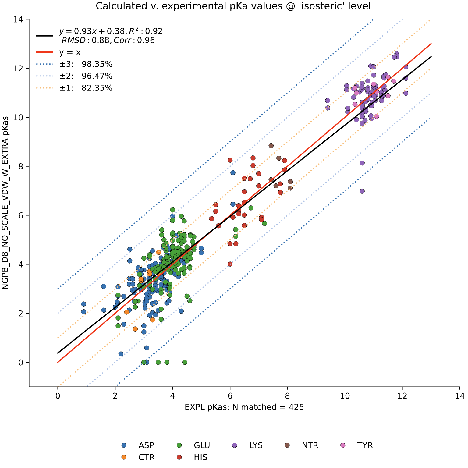
In this graph the experimental pKa values are on the X-axis and the MCCE-predicted pKa values on the Y-axis. This particular run incorporates extra values, which are residue-type-specific adjustments applied after the initial pKa calculations. These adjustments shift all predicted pKas of a given residue type uniformly up or down to reduce systematic bias. However, it's important to note that while extra values can correct for bias, they do not address the variance within a residue group relative to experimental values.

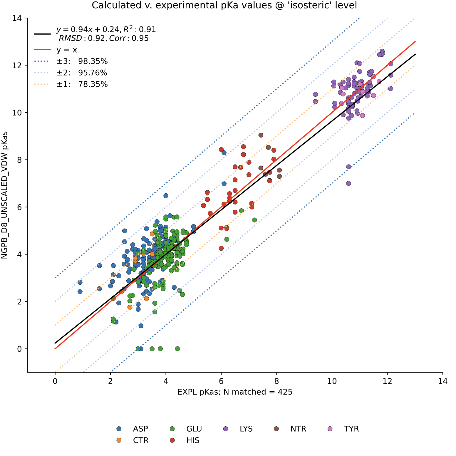
For comparison, the following graph shows the same dataset without applying extra values. Here, we observe the pKa accuracy was reduced by 4% to 78.35% and an inflated RMSD of 0.92.

Poisson-Boltzmann Solvers

MCCE4 is currently capable of switching between three different Poisson-Boltzmann solvers: ZAP (OpenEye), Delphi, and Next-Generation Poisson Boltzmann (NGPB created by partners in the CONCEPT Lab @ Istituto Italiano di Tecnologia (ITT) in conjunction with Gunner Lab). 

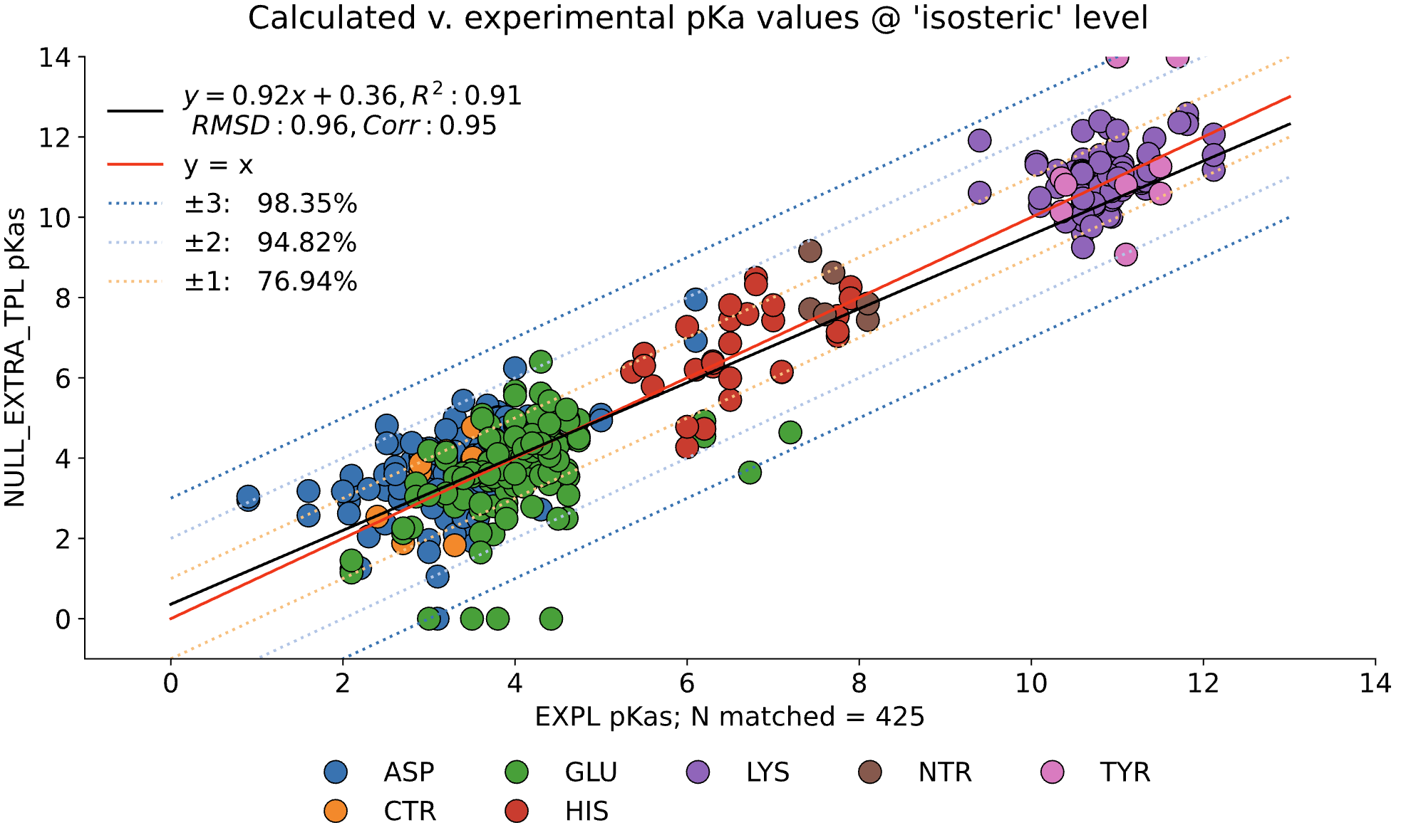
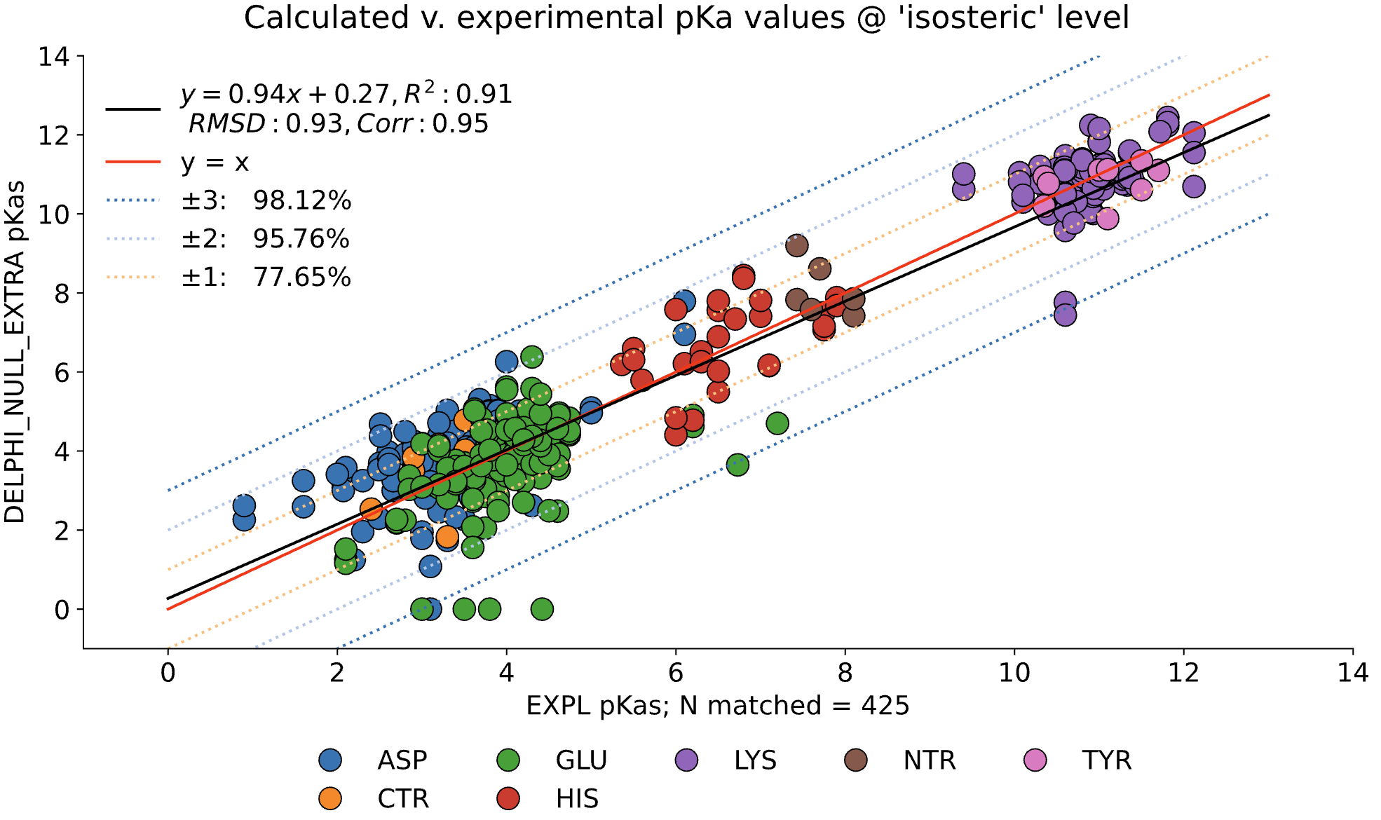
Here, we examine the pKa accuracy of our three solvers on our testing set. These are implicit solvent runs, using ε=8, and modified unscaled VDW equations (see below). We have removed all "extra" terms for these graphs, so we are only seeing the solvers and MCCE's calculations in the final output. This highlights the consistency of MCCE between the different solvers. ZAP is typically the fastest solver, however as it requires a special license from OpenEye, we anticipate NGPB will be support most users' pKa calculation needs. 

NGPB

ZAP

Delphi

Dielectric Constant (ε)

MCCE output shows significant variance depending on the inner dielectric constant (ε).

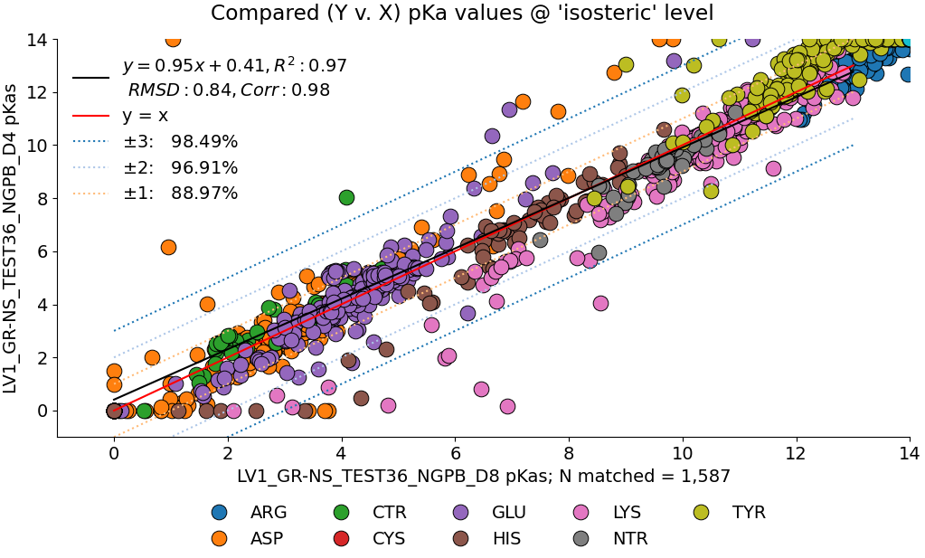
Below, we compare the optimized results from two dry NGPB runs: the left with ε=4 , and the right ε=8. Both runs use unscaled modified Van der Waals equations. The different residue groups are distributed similarly, but the ε=4 runs experience a greater variance, especially for the 425 residues with experimental data.

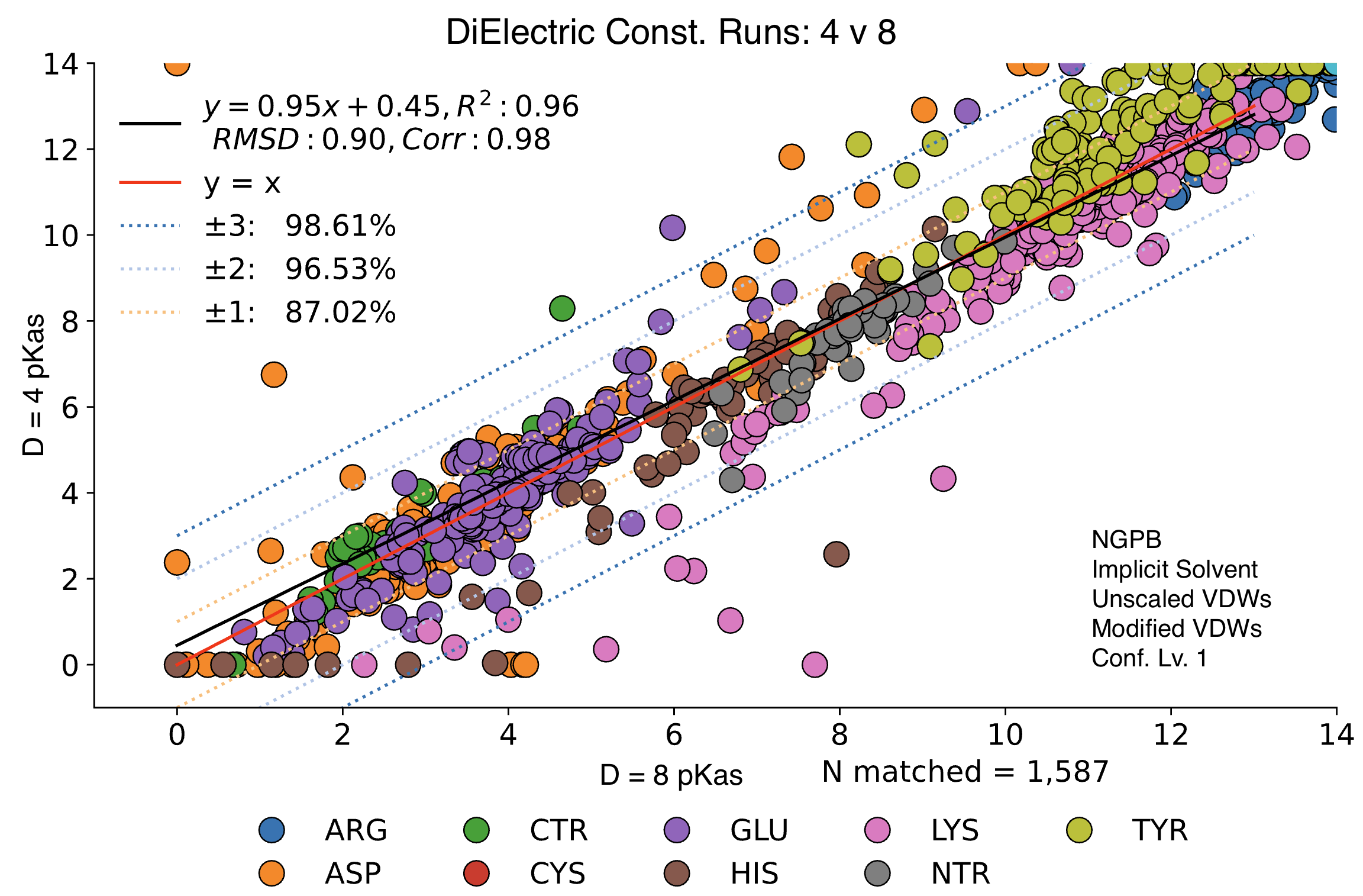
Directly comparing these two runs across all 1,587 residues, we find an average delta mean  of -.02, and an average absolute delta mean of .42. Let's look at this direct comparison: Note the legend residue color is different from previous graphs. 

Explicit vs. Implicit Solvent Runs

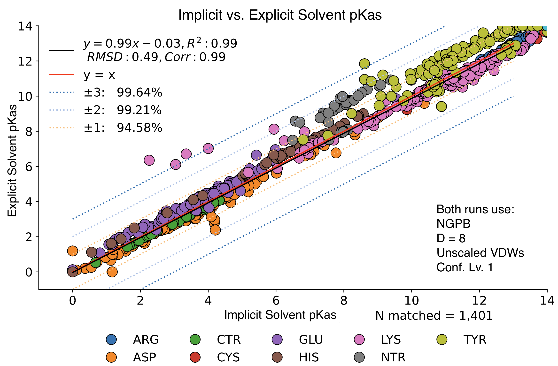
We observed little change in pKa accuracy when waters are removed from the input PDB. If no explicit waters are present in a PDB file, MCCE will assume an implicit solvent and run accordingly. Implicit runs enjoy slightly better accuracy vs. explicit runs.

In this graph, we see minimal changes in pKa calculation between wet and dry runs of NGPB for ε=8. Note that this is simply a strict comparison of calculations for across all residues between a wet and dry run, not just the experimental data. 

Traditional VDW vs Modified VDW 

Traditional van der Waals (Lennard-Jones):

The traditional van der Waals (Lennard-Jones) potential for modeling interactions between atoms is given by:

\[
V_{\text{LJ}} = \epsilon \left[ \left( \frac{r_0}{r} \right)^{12} - 2 \left( \frac{r_0}{r} \right)^6 \right]
\]

where:

- \( V_{\text{LJ}} \) = van der Waals (Lennard-Jones) potential energy  
- \( \epsilon \) = depth of the potential well (interaction strength)  
- \( r_0 \) = equilibrium distance (distance at which the potential is minimum/transition point between two regions)  
- \( r \) = distance between two interacting particles

Modified van der Waals (Lennard-Jones):

Our modified van der Waals (Lennard-Jones) potential introduces a piecewise form to replace the standard Lennard-Jones (LJ) potential near short distances: 

\[
\begin{align}
V_{\text{LJ}_{\text{mod}}} =\ & \Theta(r_0 - r) \left[ \epsilon \left( \ln\left( \frac{r_0}{r} \right) \left( \frac{r_0}{r} \right)^p \right) - \epsilon \right] \nonumber \\
& +\ \Theta(r - r_0)\ \epsilon \left[ \left( \frac{r_0}{r} \right)^{12} - 2 \left( \frac{r_0}{r} \right)^6 \right]
\end{align}
\]

where:

- \( V_{\text{LJ}_{\text{mod}}} \) = Modified van der Waals (Lennard-Jones) potential energy
- \( \epsilon \) = depth of the potential well (interaction strength)  
- \( r_0 \) = equilibrium distance (distance at which the potential is minimum/transition point between two regions)  
- \( p \) = adjustable exponent for the repulsive region \( (r < r_0) \)  (default: 6)
- \( r \) = distance between two interacting particles  
- \( \Theta \) = Heaviside step function:
- \( \Theta(x) = 1 \) if \( x > 0 \), and \( \Theta(x) = 0 \) otherwise

Comparison of Standard and Modified van der Waals (Lennard-Jones) Potentials

In the standard Lennard-Jones (LJ) potential:

\[
V_{\text{LJ}} = 4 \epsilon \left[ \left( \frac{\sigma}{r} \right)^{12} - \left( \frac{\sigma}{r} \right)^6 \right]; \quad \sigma = \frac{r_0}{\sqrt[6]{2}}
\]

- The repulsive term \( r^{-12} \), diverges very steeply as \( r \to 0 \), leading to extremely large energies that can cause instability or poor numerical behavior in molecular simulations.
-  \( \sigma \) is the characteristic distance parameter of the potential. The potential minimum occurs at the distance r_0​.
- For \( r < \sigma \), the force becomes strongly repulsive.

In contrast, our modified potential \( V_{\text{LJ}_{\text{mod}}} \) has the following key differences:

Piecewise Definition

- For short distances \( r < r_0 \), the standard repulsive \( r^{-12} \) term is replaced by a smoother, logarithmic form:

\[
\epsilon \left( \ln\left( \frac{r_0}{r} \right) \left( \frac{r_0}{r} \right)^p \right) - \epsilon
\]

- This reduces the divergence of the potential at very short distances and provides a more controllable repulsive wall, which can improve numerical stability and physical realism.

Matching to Standard LJ at Larger Distances

- For longer distances \( r \geq r_0 \), the potential smoothly transitions back to a standard Lennard-Jones attractive tail:

\[
\epsilon \left[ \left( \frac{r_0}{r} \right)^{12} - 2 \left( \frac{r_0}{r} \right)^6 \right]
\]

Tunable Repulsive Behavior

- The exponent \( p \) in the short-distance repulsive form allows for tuning the shape and steepness of the repulsive wall which is not possible in the fixed standard LJ potential.

Improved Physical Behavior

- The modified potential avoids unphysically large energies for particles approaching very short distances (which can happen due to numerical noise or flexible molecules).
- The logarithmic form provides a softer repulsive barrier, which can better model interactions in crowded or soft systems (e.g., water near hydrophobic surfaces, flexible molecules, proteins).

Summary

Standard LJ	Modified \( V_{\text{LJ}_{\text{mod}}} \)
Single analytic form	Piecewise form (logarithmic + LJ)
Strong divergence at short distances	Smooth repulsive wall at short distances
No tuning of repulsion	Adjustable repulsion via parameter \( p \)
Simpler but harsher behavior	More numerically stable, physically motivated behavior

Modified VDW Raw Information

For your perusal, we include this chart of various runs. The Amino Acid columns are a count of how many pKas were outside of -/+2 units from the experimental- outliers of each residue type.

Residue Totals Across Experimental PDBs

Res. Totals	ARG	ASP	CTR	GLU	HIS	LYS	NTR	TYR	Sum
Num. Res.	243	287	56	236	66	378	51	259	1576
Num. Experimental pKas	0	147	10	147	29	77	6	9	425

Outlier Residues of Various Runs

Solver	D	Dry	Level	ASP	GLU	HIS	LYS	NTR	TYR	Sum	pKa Acc.	RMSD	RMSD (w/o outliers)
Delphi	4	Dry	1	10	19	4	2	2	1	38		1.34	.84
Delphi	8	Dry	1	7	7	0	3	2	0	19		.97	.76
Delphi	4	Wet	1	14	20	4	2	2	1	43		1.34	.85
Delphi	8	Wet	1	7	6	1	0	2	0	16		.93	.76
NGPB	4	Dry	1	16	15	3	3	2	2	41		1.28	.8
NGPB	8	Dry	1	6	6	2	2	2	0	18		.95	.73
NGPB	4	Wet	1	14	18	3	4	2	2	43		1.3	.81
NGPB	8	Wet	1	7	5	1	2	2	0	17		.98	.77
Zap	4	Dry	1	24	21	7	4	0	1	57		1.43	.88
Zap	8	Dry	1	5	8	2	0	2	0	17		.95	.76
Zap	4	Wet	1	16	19	4	4	1	1	45		1.3	.82
Zap	8	Wet	1	7	9	2	2	2	0	22		.99	.74
Delphi	4	Dry	2	24	29	1	6	1	2	63		1.49	.94
Delphi	8	Dry	2	5	13	3	2	2	0	14		.88	.74
NGPB	4	Dry	2	15	19	6	3	0	0	43		1.7	.81
NGPB	8	Dry	2	6	5	1	1	1	0	14		.9	.68
Zap	4	Dry	2	21	19	6	1	0	1	49		1.31	.92
Zap	8	Dry	2	3	9	1	1	1	0	15		.88	.74

ARG and CTR residue type data was also collected, but since only few outliers were found their columns were removed for readabilty. While MCCE is capable of doing wet runs at Level 2, these take a significantly longer amount of time for a low benefit, so few such runs have been performed by the Gunner lab thus far. Note how the ε = 4 runs have consistently larger numbers of outliers, and how RMSD also suffers for the category. 

Conclusions

In conclusion, we demonstrate that for the used Benchmark PDB files, MCCE represents a robust way to estimate pKa values, showcasing consistency between solvers and other settings and conditions. ZAP remains the fastest option, but for those without a license, NGPB provides good accuracy. For most pKa findings needs, we recommend runs that use options dry, ε = 8,  conformer sampling Lvl. 1, and NGPB. If this is not sufficient, try conformer sampling Lvl. 2. 

Special thanks to the National Science Foundation, the Department of Energy, and the City College of New York for making this research possible.