Results

Findings about MCCE and its settings

• How does changing MCCE's parameters change accuracy? (under construction)
• How to break down the energy of a residue ionization?
• MCCE Output Files

How does changing MCCE's parameters change accuracy? (under construction)

MCCE offers a wide range of customizable parameter that influence the accuracy of its pKa predictions. Some major options include varying the internal dielectric constants, numerical Poisson-Boltzmann solvers, Van der Waal functions, conformer sampling level, and explicit crystal water inclusion/removal (implicit/explicit). Each of these options or combinatoric assortments of these options can significantly impact MCCE's free energy model, and in turn, affects its pKa predictions. In this study, we systematically evaluate how these parameter choices affect MCCE's calculated pKa values against experimental benchmark values. 

Here, we use a set of 36 PDB files sourced from RCSB.org, see PDB Benchmark Files.txt. These PDB files were chosen for their varying sizes, as well as the amount of experimental data available for their residue pKa values. You can find the sources for the experimental pKas in this file: pkdbv1_WT_pkas.csv (change this later to be a citation probably)

Note that the starting and ending residues of protein chains are re-named to NTR and CTR, respectively. At time of writing, MCCE will re-label the first and last residue of a chain, even if the input structure is incomplete.

Accuracy Criteria

Our benchmark dataset consists of 36 PDB files comprising a total of 1,587 residues, of which 425 have experimentally verified pKa values. These will serve as our reference for evaluating the accuracy of MCCE’s pKa predictions. To perform this evaluation, we developed an in-house program that runs parallel MCCE simulations across the 36 structures and compares the predicted pKa values to the experimental values.

We define pKa Accuracy as the percentage of predicted pKa values that fall within ±1 pH unit of the corresponding experimental values. We report the root-mean-square deviation (RMSD), noting that it is sensitive to outliers; where appropriate, we assess how removing outliers affects this metric. The higher the pKa Accuracy is, and the lower the RMSD is, the better the run. 

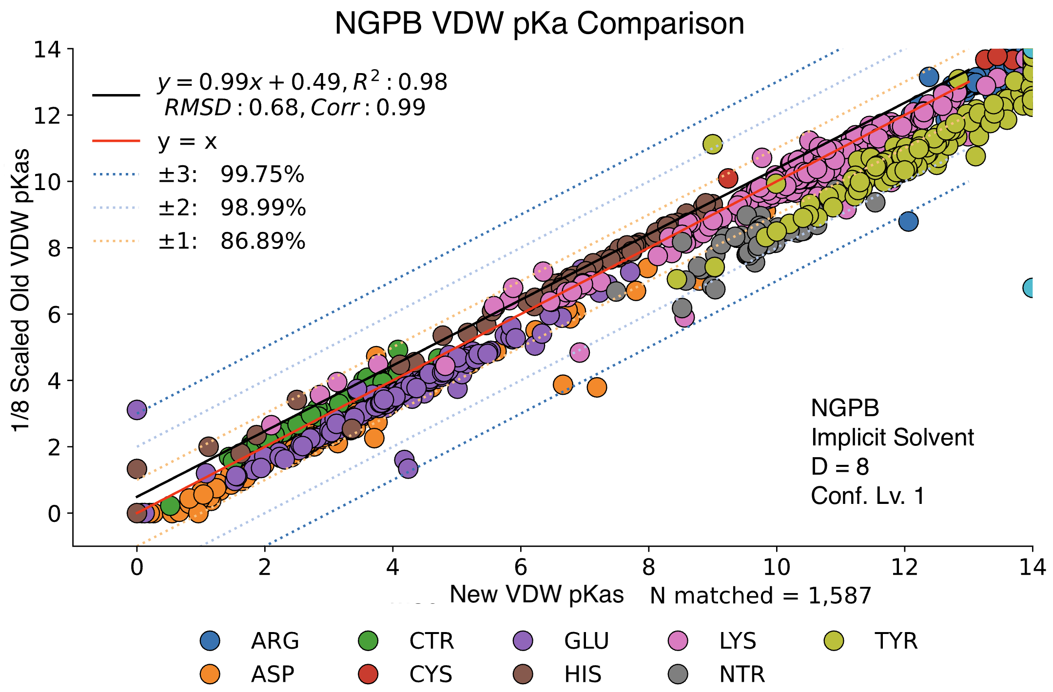
The data presented below were generated using the NGPB Poisson–Boltzmann solver with an internal dielectric constant of 8 and our modified, unscaled van der Waals function. Under these conditions, we observed a pKa Accuracy of 82.35% and an RMSD of 0.88.

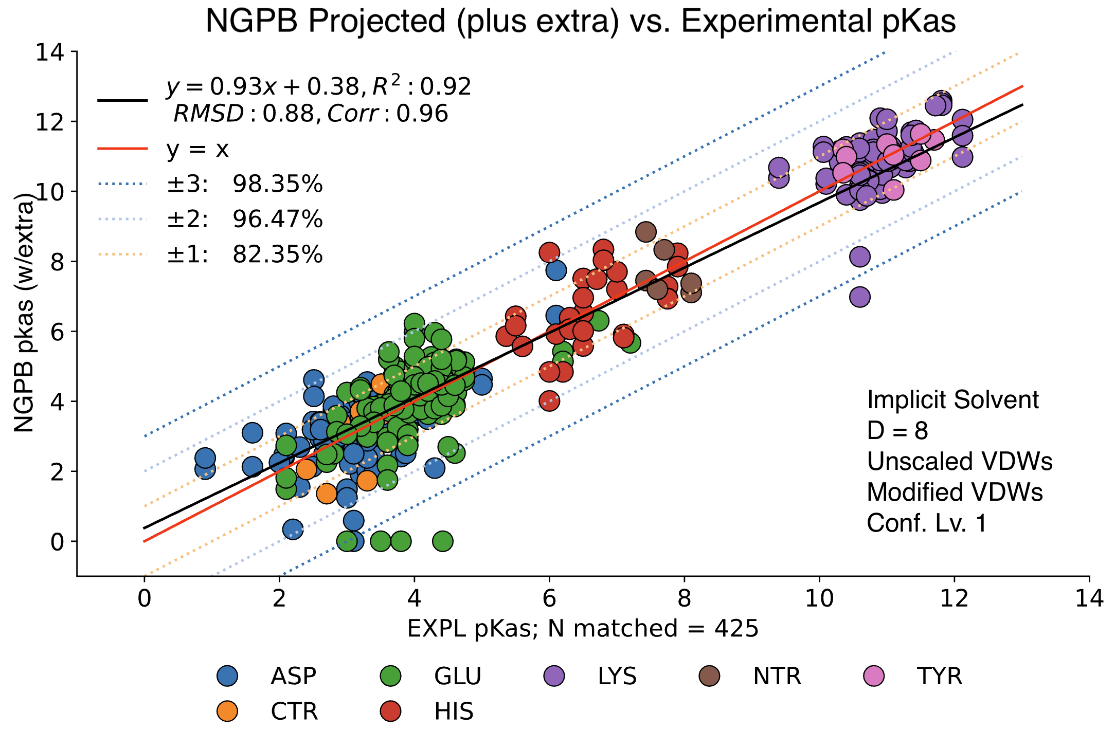
In this graph the experimental pKa values are on the X-axis and the MCCE-predicted pKa values on the Y-axis. This particular run incorporates extra values, which are residue-type-specific adjustments applied after the initial pKa calculations. These adjustments shift all predicted pKas of a given residue type uniformly up or down to reduce systematic bias. However, it's important to note that while extra values can correct for bias, they do not address the variance within a residue group relative to experimental values.

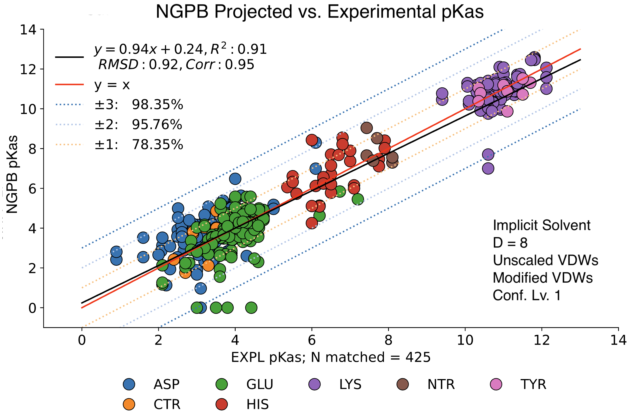
For comparison, the following graph shows the same dataset without applying extra values. Here, we observe the pKa accuracy was reduced by 4% to 78.35% and an inflated RMSD of 0.92.

Stochastic Variation Between Runs

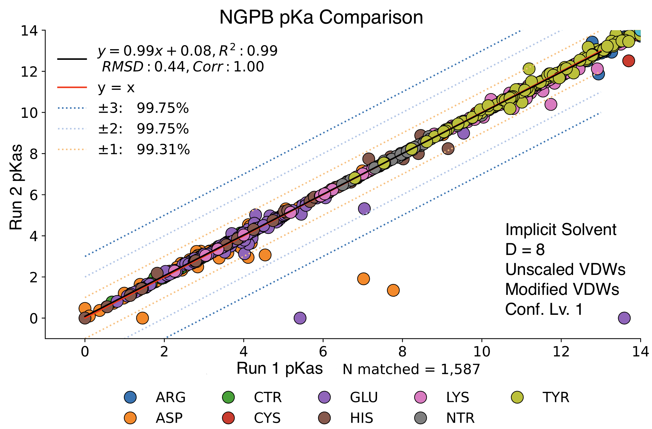
Steps 2 and 4 of MCCE incorporate randomness. For step 2, MCCE keeps rotamers that pass energy clash and steric filters, using a randomized exploration of conformational space. Due to the energy minimization, it's typical that very similar conformers are kept between two different runs. Step 4 features Monte Carlo calculations where millions of random conformers are proposed, and moves are accepted or rejected using the Metropolis criterion. Millions of microstates are accepted, so it's expected to see minimal random variation between runs. Below we see a direct comparison of two NGPB runs with identical settings. The vast majority of pKas are practically identical, though a few notable exceptions have failed to converge. While random chance does play a role in the final pKa calculation, most of the differences we will observe in future comparisons can be explained by differences in parameter choice.

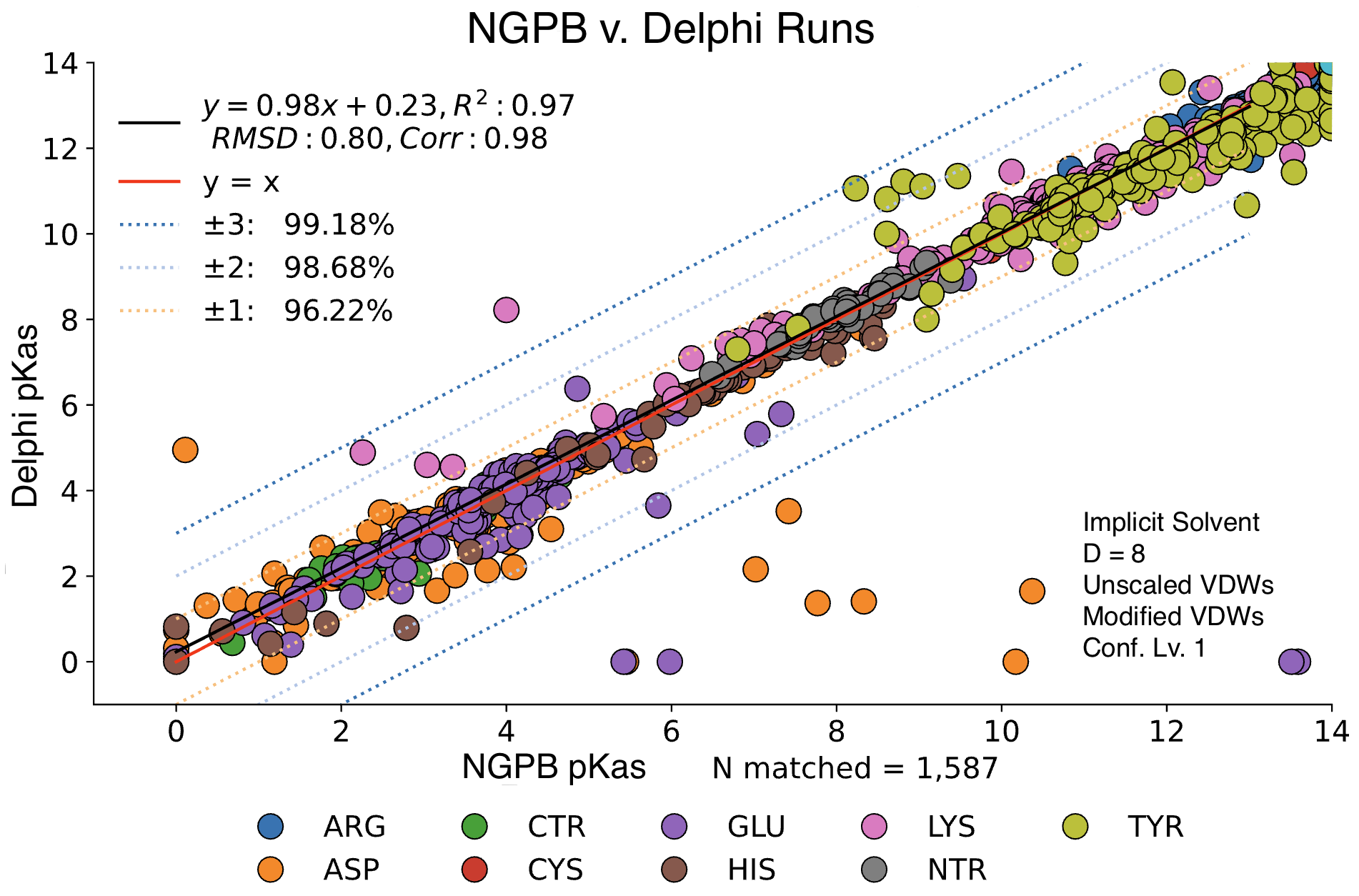
Poisson-Boltzmann Solvers

MCCE4 is currently capable of switching between three different Poisson-Boltzmann solvers: ZAP (OpenEye), Delphi, and Next-Generation Poisson Boltzmann (NGPB created by partners in the CONCEPT Lab @ Istituto Italiano di Tecnologia (ITT) in conjunction with Gunner Lab). 

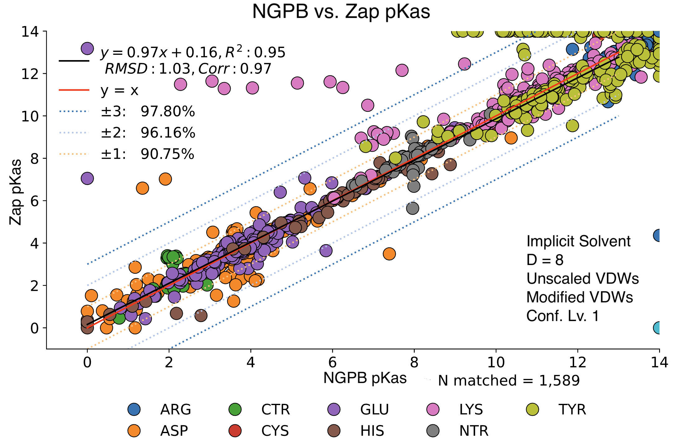
Here, we examine the pKa accuracy of our three solvers on our testing set. These are implicit solvent runs, using ε=8, and modified unscaled VDW equations (see below). We have removed all "extra" terms for these graphs, so we are only seeing the solvers and MCCE's calculations in the final output. This highlights the consistency of MCCE between the different solvers. ZAP is typically the fastest solver, however as it requires a special license from OpenEye, we anticipate NGPB will be support most users' pKa calculation needs. 

Dielectric Constant (ε)

MCCE output shows significant variance depending on the inner dielectric constant (ε).

Below, we compare the optimized results from two dry NGPB runs: the left with ε=4 , and the right ε=8. Both runs use unscaled modified Van der Waals equations. The different residue groups are distributed similarly, but the ε=4 runs experience a greater variance, especially for the 425 residues with experimental data.

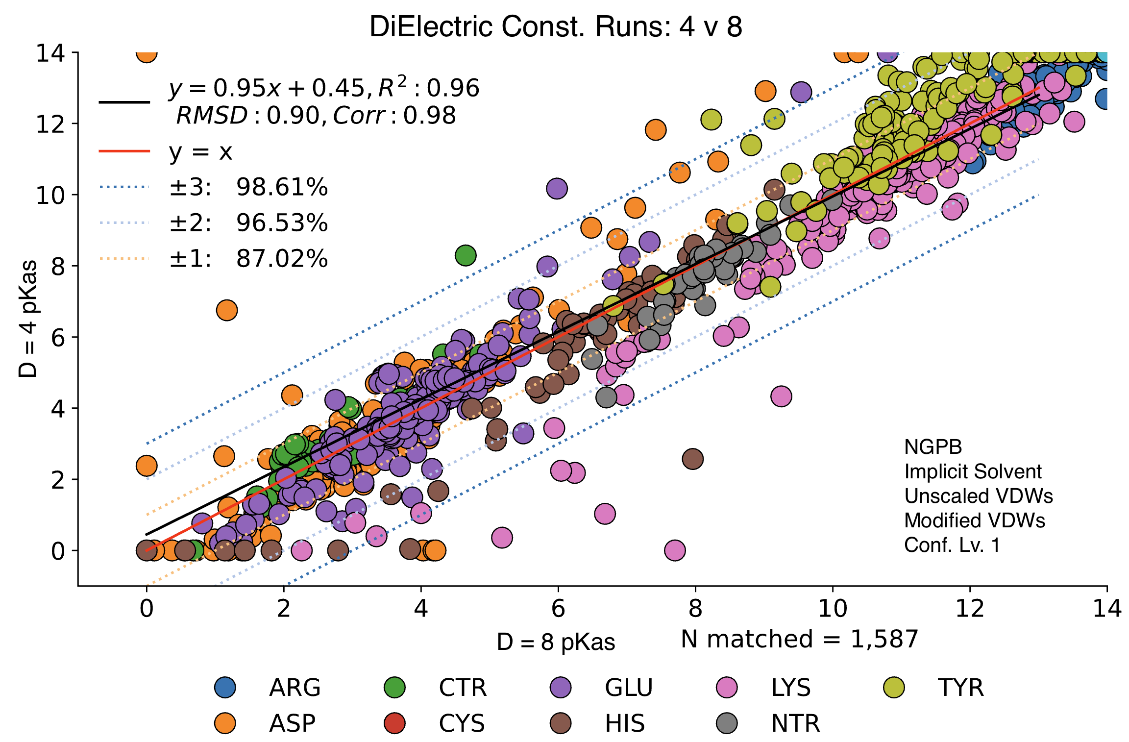
Directly comparing these two runs across all 1,587 residues, we find an average delta mean  of -.02, and an average absolute delta mean of .42. Let's look at this direct comparison: Note the legend residue color is different from previous graphs. 

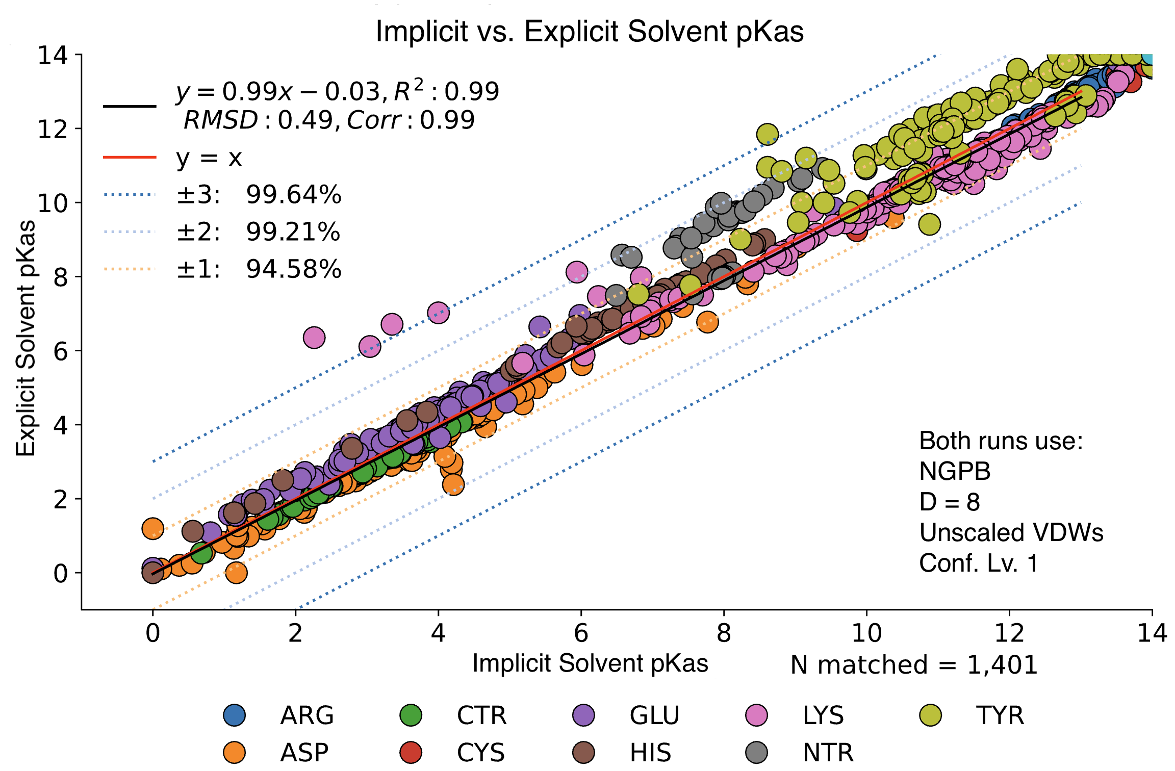
Explicit vs. Implicit Solvent Runs

We observed little change in pKa accuracy when waters are removed from the input PDB. If no explicit waters are present in a PDB file, MCCE will assume an implicit solvent and run accordingly. Implicit runs enjoy slightly better accuracy vs. explicit runs.

In this graph, we see minimal changes in pKa calculation between wet and dry runs of NGPB for ε=8. Note that this is simply a strict comparison of calculations for across all residues between a wet and dry run, not just the experimental data. 

Impact of On-The-Fly Computations

Another possible option, for step 3 of MCCE, is "--fly". Typically, desolvation energy is computed by performing a single Poisson-Boltzmann Equation run in the mixed dielectric environment and subtracting a precomputed reaction field energy value. However, this approach becomes inaccurate when the side chain conformation changes and partial charges- especially on surface Hydrogen atoms- shift, since the precomputed reference energy (stored in the ftpl file) is fixed, and does not account for such conformational variation.

The "--fly" flag improves this by computing the reference reaction field energy dynamically, or "on-the-fly". For each conformer, both the reference and in-protein reaction field energies are calculated freshly. The desolvation energy is then obtained as the difference between these two values, making the result less sensitive to changes in conformer orientation.

 

Traditional VDW vs Modified VDW 

Traditional van der Waals (Lennard-Jones):

The traditional van der Waals (Lennard-Jones) potential for modeling interactions between atoms is given by:

\[
V_{\text{LJ}} = \epsilon \left[ \left( \frac{r_0}{r} \right)^{12} - 2 \left( \frac{r_0}{r} \right)^6 \right]
\]

where:

- \( V_{\text{LJ}} \) = van der Waals (Lennard-Jones) potential energy  
- \( \epsilon \) = depth of the potential well (interaction strength)  
- \( r_0 \) = equilibrium distance (distance at which the potential is minimum/transition point between two regions)  
- \( r \) = distance between two interacting particles

Modified van der Waals (Lennard-Jones):

Our modified van der Waals (Lennard-Jones) potential introduces a piecewise form to replace the standard Lennard-Jones (LJ) potential near short distances: 

\[
\begin{align}
V_{\text{LJ}_{\text{mod}}} =\ & \Theta(r_0 - r) \left[ \epsilon \left( \ln\left( \frac{r_0}{r} \right) \left( \frac{r_0}{r} \right)^p \right) - \epsilon \right] \nonumber \\
& +\ \Theta(r - r_0)\ \epsilon \left[ \left( \frac{r_0}{r} \right)^{12} - 2 \left( \frac{r_0}{r} \right)^6 \right]
\end{align}
\]

where:

- \( V_{\text{LJ}_{\text{mod}}} \) = Modified van der Waals (Lennard-Jones) potential energy
- \( \epsilon \) = depth of the potential well (interaction strength)  
- \( r_0 \) = equilibrium distance (distance at which the potential is minimum/transition point between two regions)  
- \( p \) = adjustable exponent for the repulsive region \( (r < r_0) \)  (default: 6)
- \( r \) = distance between two interacting particles  
- \( \Theta \) = Heaviside step function:
- \( \Theta(x) = 1 \) if \( x > 0 \), and \( \Theta(x) = 0 \) otherwise

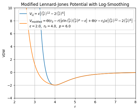
Comparison of Standard and Modified van der Waals (Lennard-Jones) Potentials

In the standard Lennard-Jones (LJ) potential:

\[
V_{\text{LJ}} = 4 \epsilon \left[ \left( \frac{\sigma}{r} \right)^{12} - \left( \frac{\sigma}{r} \right)^6 \right]; \quad \sigma = \frac{r_0}{\sqrt[6]{2}}
\]

• The repulsive term \( r^{-12} \), diverges very steeply as \( r \to 0 \), leading to extremely large energies that can cause instability or poor numerical behavior in molecular simulations.
• \( \sigma \) is the characteristic distance parameter of the potential. The potential minimum occurs at the distance \( r_{0} \).
• For \( r < \sigma \), the force becomes strongly repulsive.

In contrast, our modified potential \( V_{\text{LJ}_{\text{mod}}} \) has the following key differences:

For short distances \( r < r_0 \), the standard repulsive \( r^{-12} \) term is replaced by a smoother, logarithmic form:

\[
\epsilon \left( \ln\left( \frac{r_0}{r} \right) \left( \frac{r_0}{r} \right)^p \right) - \epsilon
\]

• This reduces the divergence of the potential at very short distances and provides a more controllable repulsive wall, which can improve numerical stability and physical realism.

For longer distances \( r \geq r_0 \), the potential smoothly transitions back to a standard Lennard-Jones attractive tail:

\[
\epsilon \left[ \left( \frac{r_0}{r} \right)^{12} - 2 \left( \frac{r_0}{r} \right)^6 \right]
\]

Tunable Repulsive Behavior: The exponent \( p \) in the short-distance repulsive form allows for tuning the shape and steepness of the repulsive wall which is not possible in the fixed standard LJ potential.

Improved Physical Behavior

• The modified potential avoids unphysically large energies for particles approaching very short distances (which can happen due to numerical noise or flexible molecules).
• The logarithmic form provides a softer repulsive barrier, which can better model interactions in crowded or soft systems (e.g., water near hydrophobic surfaces, flexible molecules, proteins).

Summary

Standard LJ	Modified \( V_{\text{LJ}_{\text{mod}}} \)
Single analytic form	Piecewise form (logarithmic + LJ)
Strong divergence at short distances	Smooth repulsive wall at short distances
No tuning of repulsion	Adjustable repulsion via parameter \( p \)
Simpler but harsher behavior	More numerically stable, physically motivated behavior

Modified VDW Raw Information

For your perusal, we include this chart of various runs. The Amino Acid columns are a count of how many pKas were outside of -/+2 units from the experimental- outliers of each residue type.

Residue Totals Across Experimental PDBs

Res. Totals	ARG	ASP	CTR	GLU	HIS	LYS	NTR	TYR	Sum
Num. Res.	243	287	56	236	66	378	51	259	1576
Num. Experimental pKas	0	147	10	147	29	77	6	9	425

Outlier Residues of Various Runs

Solver	D	Dry	Level	ASP	GLU	HIS	LYS	NTR	TYR	Sum	pKa Acc.	RMSD	RMSD (w/o outliers)
Delphi	4	Dry	1	10	19	4	2	2	1	38	69%	1.34	.84
Delphi	8	Dry	1	7	7	0	3	2	0	19	77%	.97	.76
Delphi	4	Wet	1	14	20	4	2	2	1	43	67%	1.34	.85
Delphi	8	Wet	1	7	6	1	0	2	0	16		.93	.76
NGPB	4	Dry	1	16	15	3	3	2	2	41	72%	1.28	.8
NGPB	8	Dry	1	6	6	2	2	2	0	18	78%	.95	.73
NGPB	4	Wet	1	14	18	3	4	2	2	43	70%	1.3	.81
NGPB	8	Wet	1	7	5	1	2	2	0	17	77%	.98	.77
Zap	4	Dry	1	24	21	7	4	0	1	57	62%	1.43	.88
Zap	8	Dry	1	5	8	2	0	2	0	17	76%	.95	.76
Zap	4	Wet	1	16	19	4	4	1	1	45	68%	1.3	.82
Zap	8	Wet	1	7	9	2	2	2	0	22	77%	.99	.74
Delphi	4	Dry	2	24	29	1	6	1	2	63	75%	1.49	.94
Delphi	8	Dry	2	5	13	3	2	2	0	14		.88	.74
NGPB	4	Dry	2	15	19	6	3	0	0	43	66%	1.7	.81
NGPB	8	Dry	2	6	5	1	1	1	0	14	76%	.9	.68
Zap	4	Dry	2	21	19	6	1	0	1	49	55%	1.31	.92
Zap	8	Dry	2	3	9	1	1	1	0	15	72%	.88	.74

ARG and CTR residue type data was also collected, but since only few outliers were found their columns were removed for readabilty. While MCCE is capable of doing wet runs at Level 2, these take a significantly longer amount of time for a low benefit, so few such runs have been performed by the Gunner lab thus far. Note how the ε = 4 runs have consistently larger numbers of outliers, and how RMSD also suffers for the category. 

Conclusions

In conclusion, we demonstrate that for the used Benchmark PDB files, MCCE represents a robust way to estimate pKa values, showcasing consistency between solvers and other settings and conditions. ZAP remains the fastest option, but for those without a license, NGPB provides good accuracy. For most pKa findings needs, we recommend runs that use options dry, ε = 8,  conformer sampling Lvl. 1, and NGPB. If this is not sufficient, try conformer sampling Lvl. 2. Using the --fly tag on step 3, for dynamic reference reaction field energy computation, can also reduce variance in the final calculation.

Special thanks to the National Science Foundation, the Department of Energy, and the City College of New York for making this research possible. 

How to break down the energy of a residue ionization?

How to break down the energy of a residue ionization?

MCCE calculates theoretical pKas as well as explain why these residues have those pKas.

Continuum Electrostatic interpretation of pKa

Free energy and pKa

An amino acid and conjugate base in equilibrium:

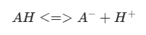
The free energy of the reaction has relationship with the equilibrium of:

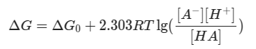
At the equilibrium of midpoint where

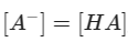
therefore residue pKa is linked to the reaction free energy:

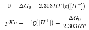
The acids in solution and in protein

We know the ionization energy in solution, which is represented by the solution pKa:

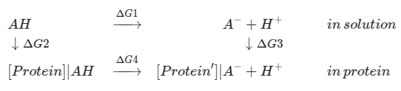
$\Delta \mathrm{G1}$ is solution pKa, and $\Delta G4$ is acid pKa in protein, what we are looking for. $\Delta G2$ and $\Delta G3$ involve the free energy of moving acid from solution to protein environment, interaction between the acid and the protein, and the interaction within the protein at $AH$ and $A^{-}$ states.

The desolvation energy, pairwise interactions are all calculated by continuum electrostatic methods.

MCCE's way to compute pKa

MCCE makes residues as independently ionizable pieces. All residues are given freedom to change conformation and ionization if possible. Residue pairwise interactions are precalculated. The choice of a residue being at which position and ionization state is statistically counted by Monte Carlo sampling.

A pKa calculation is a simulated titration that carried out at multiple pH points. The residue charges change with pH, and their pKas are their midpoints determined by fitting the titration curve.

Therefore the calculated pKa of a residue is a statistical result that came from the simultaneous interactions of many factors. To understand the pKa, we need to decipher the factors with the help of mean field energy analysis.

Understanding the residue pKa and factors that affect pKa

Mean field approximation

The accurate interaction calculation is only possible at microstate level. At the end, what we know is the probability of a residue being at certain conformation and ionization.
The interaction between residues calculated after Monte Carlo sampling os approximated by "mean field".

For example, 4 possible interactions for a pair of acids could be:

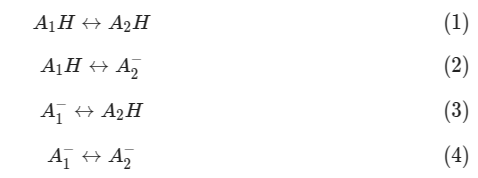
If MCCE sampled acids $A1$ and $A2$ are both at 50% ionization, after MOnte Carlo sampling, from the ionization rate alone, we could not know the interaction is 50% of (2) and 50% of (3), 50% of (1) and 50% of (4), or a mix.

This is the limitation of mean fields energy analysis. Once we know the limitation, we can extract quite useful information of residue ionization.

MFE energy terms

Once step 4 is done, one can run mfe.py on a residue to break down the energy terms of a ionization free energy. The input residue has to be in file pK.out.

For example, in lysozyme pKa calculation, we obtained pKa output file pK.out.

$ cat pK.out 
  pH             pKa/Em  n(slope) 1000*chi2      vdw0    vdw1    tors    ebkb    dsol   offset  pHpK0   EhEm0    -TS   residues   total
NTR+A0001_        5.095     0.985     0.015     -0.00   -0.01   -0.26    0.52    4.01   -0.95   -2.90    0.00    0.00   -0.11      0.29
LYS+A0001_        9.593     0.998     0.027     -0.00   -0.00    0.00    0.15    0.46    0.29   -0.81    0.00   -0.00   -0.09      0.00
ARG+A0005_       12.695     0.858     0.051     -0.01   -0.00   -0.00   -0.73    0.89    0.00    0.20    0.00    0.14   -0.35      0.14
GLU-A0007_        3.192     0.944     0.010     -0.01    0.00   -0.19   -1.27    1.17   -0.22    1.56    0.00    0.30   -1.02      0.31
LYS+A0013_       11.322     0.954     0.019     -0.00   -0.00    0.00    0.19    0.61    0.29    0.92    0.00    0.00   -2.01      0.00
ARG+A0014_       13.330     0.934     0.004     -0.01   -0.00    0.00    0.07   -0.28    0.00    0.83    0.00    0.43   -0.60      0.44
HIS+A0015_        6.816     0.988     0.065     -0.01   -0.01    0.00    1.44    1.33   -0.73   -0.16    0.00    0.36   -0.42      1.80
ASP-A0018_        2.013     0.929     0.127     -0.01   -0.00   -0.16   -2.03    0.95   -0.62    2.74    0.00    0.40   -0.86      0.40
TYR-A0020_       13.498     0.687     0.401      0.00    0.00    0.00    0.24    3.29   -0.37   -3.30    0.00    0.18    0.04      0.09
ARG+A0021_       13.239     0.796     0.092     -0.01   -0.00    0.00   -0.09    0.11    0.00    0.74    0.00    0.28   -0.74      0.29
TYR-A0023_       10.312     0.863     0.020      0.00    0.00    0.00   -1.17    1.98   -0.37   -0.11    0.00    0.29   -0.33      0.29
LYS+A0033_       10.581     0.974     0.026     -0.00   -0.00    0.00    0.06    0.61    0.29    0.18    0.00    0.00   -1.09      0.05
GLU-A0035_        5.133     0.880     1.144     -0.04   -0.01   -0.01   -1.26    2.16   -0.22   -0.38    0.00    0.26   -0.23      0.26
ARG+A0045_       12.919     0.796     1.608     -0.03   -0.00    0.00    0.19   -0.32    0.00    0.42    0.00    0.45   -0.24      0.46
ASP-A0048_        1.528     0.963     0.058     -0.01    0.00   -0.24   -2.52    3.22   -0.62    3.22    0.00    0.14   -3.01      0.17
ASP-A0052_        3.330     0.859     0.170     -0.01    0.00   -0.10   -1.32    1.99   -0.62    1.42    0.00    0.46   -1.20      0.61
TYR-A0053_        >14.0                          0.00    0.00    0.00   -1.70    4.45   -0.37   -3.80    0.00    0.00    8.03      6.61
ARG+A0061_        >14.0                         -0.01   -0.00    0.00    0.69    0.15    0.00    1.50    0.00    0.42   -2.43      0.31
ASP-A0066_        2.066     3.239     0.002     -0.01    0.02   -0.04   -5.30    7.34   -0.62    2.68    0.00   -0.11   -4.50     -0.55
ARG+A0068_       13.604     0.768     0.028      0.12    1.81    0.16    0.29   -0.80    0.00    1.10    0.00   -0.19   -0.05      2.46
ARG+A0073_       12.750     0.935     0.132     -0.01   -0.00    0.00   -0.12    0.10    0.00    0.25    0.00    0.35   -0.22      0.35
ASP-A0087_        2.073     0.960     0.014     -0.02    0.01   -0.21   -1.88    1.24   -0.62    2.68    0.00    0.31   -1.18      0.31
LYS+A0096_       10.631     0.831     0.307     -0.00    0.00    0.00   -1.52    1.26    0.29    0.23    0.00    0.00   -0.25      0.01
LYS+A0097_       10.813     0.918     0.072     -0.00   -0.00    0.00   -0.27    0.07    0.29    0.41    0.00    0.00   -0.51     -0.00
ASP-A0101_        3.988     1.009     0.010     -0.00   -0.05   -0.10    0.04    1.15   -0.62    0.76    0.00    0.57   -1.17      0.58
ARG+A0112_       12.956     0.923     0.080     -0.01   -0.00    0.00   -0.27    0.77    0.00    0.46    0.00    0.55   -0.90      0.59
ARG+A0114_       13.257     0.968     0.050     -0.01   -0.00    0.00   -0.09   -0.29    0.00    0.76    0.00    0.34   -0.35      0.35
LYS+A0116_        9.554     0.941     0.042     -0.00   -0.00    0.00    0.12    0.43    0.29   -0.85    0.00    0.00    0.02      0.01
ASP-A0119_        3.596     1.005     0.031     -0.01    0.00   -0.24   -1.08    1.95   -0.62    1.15    0.00    0.09   -1.15      0.09
ARG+A0125_       13.083     0.915     0.005     -0.01   -0.00   -0.00    0.36   -0.18    0.00    0.58    0.00    0.45   -0.75      0.45
ARG+A0128_       13.586     0.939     0.008      0.00   -0.00    0.00    0.08   -0.81    0.00    1.09    0.00    0.45   -0.36      0.45
CTR-A0129_        2.464     0.905     0.072     -0.01   -0.01   -0.12   -0.06    1.66    0.00    1.29    0.00    0.49   -2.75      0.49

 

Now we would like to know why ASP52 has a low pKa of 3.33

$ mfe.py ASP-A0052_ -c 0.1
Residue ASP-A0052_ pKa/Em=3.33
=================================
Terms          pH     meV    Kcal
---------------------------------
vdw0        -0.01   -0.85   -0.02
vdw1         0.00    0.21    0.00
tors        -0.10   -5.89   -0.14
ebkb        -1.32  -76.87   -1.81
dsol         1.99  115.58    2.72
offset      -0.62  -36.17   -0.85
pH&pK0       1.42   82.42    1.94
Eh&Em0       0.00    0.00    0.00
-TS          0.00    0.00    0.00
residues    -1.20  -69.73   -1.64
*********************************
TOTAL        0.15    8.70    0.20  sum_crg
*********************************
ASNA0044_   -0.44  -25.31   -0.59    0.00
ARGA0045_   -0.12   -6.74   -0.16    1.00
ASNA0046_   -0.16   -9.25   -0.22    0.00
ASPA0048_    0.51   29.65    0.70   -0.96
SERA0050_    0.12    7.04    0.17    0.00
GLNA0057_    0.22   12.63    0.30    0.00
ASNA0059_   -0.99  -57.31   -1.35    0.00
ARGA0061_   -0.27  -15.65   -0.37    1.00
ASPA0066_    0.39   22.84    0.54   -1.00
ARGA0112_   -0.19  -11.15   -0.26    1.00
ARGA0114_   -0.10   -5.86   -0.14    1.00
=================================

Program computes the ionization free energy, specifically, the free energy difference between the ionized ASP and the neutral ASP.

If we don't specify pH, mfe.py uses the midpoint pH or Eh.

Energy terms:

• vdw0: Van der Waals interaction within the residue. Since the vdw interaction is similar to ionized and neutral ASP, the contribution to  of ionization is small.
• vdw1: Van der Waals interaction to the protein backbone. Again the contribution to pKa is usually small.
• tors: Side chain torsion energy. The contribution to pKa is usually small.
• ebkb: The protein backbone electrostatic interaction. The protein secondary structure especially helices have a dipole that may affect the ionized residue more than neutral form of the residue, therefore it could be a factor of pKa.
• dsolv: The desolvation energy. The ionized residue is less stabilized im protein than in solution. This makes the ionization inside protein harder and it links to a positive free energy to the reaction from neutral residue to ionized residue.
• offset: The is a system correction of pKa calibrated by benchmark. It captures the terms not counted by MCCE.
• pH&pK0: Solution pH effect to the ionization. It is environment pressure to the residue ionization. To an acid, low solution pH makes the ionization (releasing proton) easy so it contributes as a favorable energy. To a base, low pH makes ionization harder. When pH equals residue's solution pKa, the environment pH is at the balance point, where the contribution is 0.
• Eh&Em0: Environment Eh effect to redox reaction. This works similarily as pH&pK0.
• -TS: Entropy term. The number of rotamers of neutral and ionized residues generated by MCCE may be different. The effect of number of rotamers on two ionization states act like entropy. Since this may not be a desired effect, one can enable entropy correction in step 4, Monte Carlo sampling. If entropy correction is enabled in MC, the entropy effect has been eliminated and entropy should be set to 0 in MFE analysis. Program mfe.py is able to know how MC is done and handle this accordingly, or one can turn on or off in MFE manually.
• residues: Total pairwise interaction from other residues. Other residues may shift the ionization free energy depending on their dipole orentation and charge.
• TOTAL: Total free enegy of ionization reaction. It the sum of all above terms.
• Redisue breakdown: Individual residue contribution. This part is the breakdown of term residues.

At the midpoint, $\left[AH\right]=\left[A^{-}\right]$. This means conformers of and conformers of  strike a balance, and the transition energy $\Delta G$ between them is 0 under this condition. The value  in pH unit also means how far away the pKa is from the solution pH. At the midpoint,  and residue pKa is the same as envrionment pH.

In the above example, ASP52 has low pH because a pretty big stabilization from ASN59.

We can also do mfe anaylysis off the midpoint, for example at physiological pH about 7. The command option "-p 7" sets the mfe point.

$ mfe.py ASP-A0052_ -c 0.1 -p 7
Residue ASP-A0052_ pKa/Em=3.33
=================================
Terms          pH     meV    Kcal
---------------------------------
vdw0        -0.02   -0.97   -0.02
vdw1        -0.01   -0.52   -0.01
tors        -0.11   -6.30   -0.15
ebkb        -1.32  -76.59   -1.80
dsol         1.97  114.53    2.69
offset      -0.62  -36.17   -0.85
pH&pK0      -2.25 -130.60   -3.07
Eh&Em0       0.00    0.00    0.00
-TS          0.00    0.00    0.00
residues    -1.81 -105.25   -2.47
*********************************
TOTAL       -4.17 -241.87   -5.68  sum_crg
*********************************
GLUA0035_    0.85   49.08    1.15   -0.98
ASNA0044_   -1.00  -57.84   -1.36    0.00
ARGA0045_   -0.11   -6.28   -0.15    1.00
ASNA0046_   -0.85  -49.43   -1.16    0.00
ASPA0048_    0.52   30.08    0.71   -1.00
SERA0050_    0.13    7.43    0.17    0.00
GLNA0057_    0.18   10.47    0.25    0.00
ASNA0059_   -1.20  -69.75   -1.64    0.00
ARGA0061_   -0.28  -16.15   -0.38    1.00
ASPA0066_    0.40   22.96    0.54   -1.00
ARGA0112_   -0.20  -11.56   -0.27    1.00
=================================

 

We see ASP52 is surrounded by these polar residues.gets extra stabilization from ASN44 and ASN46 besides ASN59. The stabilization is bigger at pH 7. Actually the back calculated pKa is lower than titrated value , indicating extra stabilization at pH 7.

With MFE analysis, one can quickly determine what residues affect the pKa most therefore identify the influential sites.

MCCE Output Files

As part of the standard four steps, MCCE produces a number of files associated with the initial protein output. These are best understood to be members of six categories:

Input: The given PDB file. Often, MCCE programs will symbolically link the name "prot.pdb" to the input PDB file.

Output: Results of MCCE computation, to be interpreted by the user. 

Records: Preserved information about the run. 

Instructions: Files that control how MCCE runs. run.prm 

Control: "Midpoint" files to preserve information between steps.

Progress: Benchmark files to keep track of what processes are occurring, and whether the run is succeeding. 

-------

Step-by-Step Output

Program start and Initialization

Input files:

• run.prm: mcce control file
• param: parameter directory (specified in run.prm)
• extra.tpl: extra parameters. Often used to correct for bias. (optional, specified in run.prm)
• new.tpl: temporary parameter file for unrecognized cofactors. (optional, created by step 1 if unknown residues are present)

Step 1: Formatting PDB File

Input files:

• PDB file
• name.txt 
• list_rot.gold (still?)

Output files:

• acc.res: solvent accessibility of residues
• acc.atm: solvent accessibility of atoms
• new.tpl: parameter file template of unrecognized cofactors (not always created)
• head1.lst: summary of rotamer making policy of residues (optionally used by step 2? how does that work?)
• step1_out.pdb (used by step 2): 

Step 2: Making Rotamers

Input files:

• step1_out.pdb: input structure of step 2 in mcce extended PDB format
• head1.lst: rotamer making policy of residues 

Output files:

• progress.log: progress report file. Dynamically updated
• rot_stat: rotamer making statistics, dynamically updated
• head2.lst: summary of rotamers made in step 2 (optionally used by step 3)
• step2_out.pdb: step 2 output file with multiple rotamers in extended PDB format

Step 3: Calculate the Energy Lookup Table

Input files:

• step2_out.pdb: Input instructions of step 3 in MCCE extended PDB format

Output files: 

Alphabetized list

acc.atm/acc.res (Control/Output) - Gives the percent surface accessibility to the solvent of the atom/residue. Used to make rotamers. 

energies (Control) - Self and pairwise energies generated during step 3. 

entropy.out - 

err.log (Progress) - Similar to progress.log, terminal output is moved here in the event of an error. Usually empty.

fort.38 (Output) - The name is a reminder that MCCE's origins were in Fortran. 

head1.lst/head2.lst/head3.lst (Control) - head1.lst is created by step 1, and can be modified to reduce the number of conformers made in step 2. head2.lst is a summary of rotamers made in step 2. 

mc_out (Progress) - Provides details about the Monte Carlo process.

name.txt (Instructions) - The file referenced by mcce when renaming atom names, residue names, sequence number, and chain ID. 

param - How 

pK.out (Output) - Sampling across different pHs 

prot.pdb (Input) - The name MCCE often uses in reference to the original input file.

respair.lst - Records the pairwise energy for each pair of conformers.

rot_stat (Progress) - Provides statistics about rotamer creation. 

run.log (Record) - Keeps a record of terminal output from steps.

run.prm (Instructions) - Created by step 1 if not provided- grants extra control over MCCE settings. For example, by default, the pH titration occurs along whole numbers from 0 - 14. The TITR settings can be edited to reduce the range of the pH titration, increase the points of titration, and more. 

run.prm.record - Records the full run.prm details for each step. CAUTION: If different settings are used on different runs in the same direct, run.prm.record may not capture the changes to the settings. 

step0_out.pdb/step1_out.pdb/step2_out.pdb - Restructured versions of the input file. step0_out deletes any header information (e.g., the headers included in RCSB downloads of PDB files). step1_out renames residues according to a file called name.txt, including the opening and concluding residues of a sequence to NTR and CTR, respectively. step2_out.pdb expands the list to include alternative conformers as well.

sum_crg.out - Records information about the net charge of the PDB's residues at each pH titration.

vdw0.lst -